Scheduling R scripts and processes on Windows and Unix/Linux

2 new R packages were put on CRAN last week by BNOSAC (www.bnosac.be).

• One package for scheduling R scripts and processes on Windows (taskscheduleR) and
• Another package for scheduling R scripts and processes on Unix / Linux (cronR)

These 2 packages allow you to schedule R processes from R directly. This is done by passing commands directly to cron which is a basic Linux/Unix job scheduling utility or by using the Windows Task Scheduler. The packages were developed for beginning R users who are unaware of that fact that R scripts can also be run non-interactively and can be automated.

We blogged already about the taskscheduleR R package at this blog post and also here. This time we devote some more details to the cronR R package.

The cronR package allows to

• Get the list of scheduled jobs
• Remove scheduled jobs
• Add a job
  • a job is basically a script with R code which is run through Rscript
  • You can schedule tasks 'ONCE', 'EVERY MINUTE', 'EVERY HOUR', 'EVERY DAY', 'EVERY WEEK', 'EVERY MONTH' or any complex schedule
  • The task log contains the stdout & stderr of the Rscript which was run on that timepoint. This log can be found at the same folder as the R script

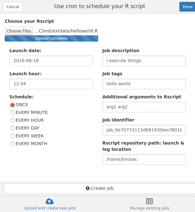
The package is especially suited for persons working on an RStudio server in the cloud or within the premises of their corporate environment. It allows to easily schedule processes. To make that extremely easy for beginning R users, an RStudio addin was developed, which is shown in the example below. The RStudio addin basically allows you to select an R script and schedule it at specific timepoints. It does this by copying the script to your launch/log folder and setting up a cronjob for that script.

The example below shows how to set up a cron job using the RStudio addin so that the scripts are launched every minute or every day at a specific hour. The R code is launched through Rscript and the log will contain the errors and the warnings in case your script failed so that you can review where the code failed.

Mark that you can also pass on arguments to the R script so that you can launch the same script for productXYZ and productABC.

Of course scheduling scripts can also be done from R directly. Some examples are shown below. More information at https://github.com/bnosac/cronR

library(cronR)
f <- system.file(package = "cronR", "extdata", "helloworld.R")
cmd <- cron_rscript(f, rscript_args = c("productx", "20160101"))
## Every minute
cron_add(cmd, frequency = 'minutely', id = 'job1', description = 'Customers')
## Every hour at 20 past the hour on Monday and Tuesday
cron_add(cmd, frequency = 'hourly', id = 'job2', at = '00:20', description = 'Weather', days_of_week = c(1, 2))
## Every day at 14h20 on Sunday, Wednesday and Friday
cron_add(cmd, frequency = 'daily', id = 'job3', at = '14:20', days_of_week = c(0, 3, 5))
## Every starting day of the month at 10h30
cron_add(cmd, frequency = 'monthly', id = 'job4', at = '10:30', days_of_month = 'first', days_of_week = '*')
## Get all the jobs
cron_ls()
## Remove all scheduled jobs
cron_clear(ask=FALSE)

We hope this will gain you some precious time and if you need more help on automating R processes, feel free to get into contact. We have a special training devoted to managing R processes which can be given in your organisation. More information at our training curriculum.

Detect Lines in Digital Images

As part of our data science training initiative, bnosac is also providing a course on computer vision with R & Python which is held in March 9-10 in Leuven, Belgium (subscribe here or have a look at our full training offer here). Part of the course is covering finding blobs, corners, gradients, edges & lines in images.

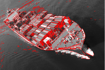
For this reason, the R package image.LineSegmentDetector was made available at https://github.com/bnosac/image. It allows to detect segment lines in digital images. An example of this is shown below.

library(image.LineSegmentDetector)
library(pixmap)

## Read in the image + make sure input to the algorithm is matrix with grey-scale values in 0-255 range
imagelocation <- system.file("extdata", "chairs.pgm", package="image.LineSegmentDetector")
image <- read.pnm(file = imagelocation, cellres = 1)
x <- image@grey * 255
## Detect and plot the lines segments
linesegments <- image_line_segment_detector(x)
linesegments
plot(image)
plot(linesegments, add = TRUE, col = "red")

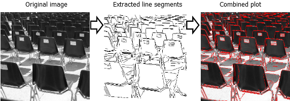
The line segment detector finds lines in digital grey-scale images and is an implementation of the linear-time Line Segment Detector explained at https://doi.org/10.5201/ipol.2012.gjmr-lsd. It gives subpixel accurate results and is designed to work on any digital image without parameter tuning. It controls its own number of false detections where on average, one false alarm is allowed per image.
More information here https://github.com/bnosac/image

The algorithm requires as input a grey-scale image. So if you have another image, you can use the excellent magick package to transform it to grey scale.

library(magick)
f <- tempfile(fileext = ".pgm")
x <- image_read("http://www.momentumshipping.net/lounge/wp-content/uploads/2015/10/containership2.jpg")
x <- image_convert(x, format = "pgm", depth = 8)
image_write(x, path = f, format = "pgm")
image <- read.pnm(file = f, cellres = 1)
linesegments <- image_line_segment_detector(image@grey * 255)
plot(image)
plot(linesegments, add = TRUE, col = "red")

The algorithm is implemented with Rcpp and is released under the AGPL-3 license. Hope you enjoy it.

Need support in image recognition? Let us know.

An overview of text mining visualisations possibilities with R on the CETA trade agreement

Text Mining has become quite mainstream nowadays as the tools to make a reasonable text analysis are ready to be exploited and give astoundingly nice and reasonable results. At BNOSAC, we use it mainly for text mining on call center data, poetry, salesforce data, emails, HR reviews, IT logged tickets, customer reviews, survey feedback and many more. We also provide training on text mining with R in Belgium (next trainings are scheduled on November 14/15 2016 and March 23/24 2017 in Belgium, to subscribe: go here or here).

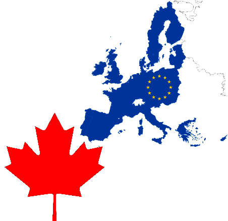
For this blog post, we will focus on the most relevant visualisations which exist in text mining by using the CETA trade agreement between the EU and Canada.

This trade agreement is available as a pdf on www.trade.ec.europa.eu/doclib/docs/2014/september/tradoc_152806.pdf and we would like to see what is written in there without having to read all of the 1598 pages in which our politicians in Belgium seem to have found good reasons to at least for a while politically block the process of signing this treaty.

Let us start by reading in the pdf file in R which is pretty easy nowadays.

library(pdftools)
library(data.table)
txt <- pdf_text("tradoc_152806.pdf")
txt <- unlist(txt)
txt <- paste(txt, collapse = " ")

Research done in 2012 (Wikipedia) showed that the average reading speed is 184 words per minute or 863 characters per minute. The CETA treaty has 3091384 characters and 334723 terms (words excluding punctuations). A quick calculation tells me that reading this document would take me between 30 and 59 hours non-stop. Were are not going to do this but instead do some text mining on the CETA treaty.

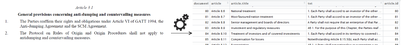
If you are doing text mining, people refer to text as part of documents. In this case there is only 1 document, the CETA treaty. For further analysis, we will assume that each article of the CETA treaty is a document. As you can see in the following screenshot, the article starts always with the word article and next some numbers. Let's extract this so that we have a dataset with 453 articles, the header and the content. The R code for this is put at https://github.com/jwijffels/ceta-txtmining/blob/master/01_import_ceta_treaty_pos_tagging.R. This dataset is available at https://github.com/jwijffels/ceta-txtmining.

A first step in text mining is always to do a Parts-of-Speech (POS) tagging. This assigns to each word a tag (noun, verb, adverb, adjective, pronoun, ...). Mostly you are only interested in nouns and some verbs and POS tagging allows you to easily do this. POS tagging for Dutch/French/English/German/Spanish/Italian can be done with the pattern.nlp package available at https://github.com/bnosac/pattern.nlp. We do this for all 453 articles in the treaty and show the distribution of the POS tags.

## Natural Language Processing: POS tagging
library(pattern.nlp)
ceta_tagged <- mapply(article.id = ceta$article.id, content = ceta$txt, FUN=function(article.id, content){
  out <- pattern_pos(x = content, language = "english", core = TRUE)
  out$article.id <- rep(article.id, times = nrow(out))
  out
}, SIMPLIFY = FALSE)  
ceta_tagged <- rbindlist(ceta_tagged)

## Take only nouns
ceta_nouns <- subset(ceta_tagged, word.type %in% c("NN") & nchar(word.lemma) > 2)

## All data in 1 list
ceta <- list(ceta_txt = txt, ceta = ceta, ceta_tagged = ceta_tagged, ceta_nouns = ceta_nouns)

## Look at POS tags
library(lattice)
barchart(sort(table(ceta$ceta_tagged$word.type)), col = "lightblue", xlab = "Term frequency", 
         main = "Parts of Speech Tag term frequency\n in CETA treaty")

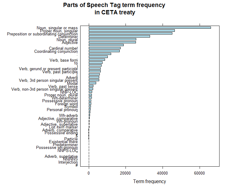
In what comes further, we only work on the nouns (POS tags NN). The data preparation for the text analysis is now done, we have a dataset with 1 row per word and the corresponding tag. We can now start to do some analysis and to make some graphs

In order to split up the 453 articles into relevant topics, we generate a topic model (code can be found here). Let's hope we find an indication that some part of the treaty will indeed cover the issues the Walloon minister president Paul Magnette was talking about. The core R code which fits this is shown below and fits a topic model with 5 topics on the top 250 terms occurring in the CETA treaty.

ceta_topics <- LDA(x = dtm[, topterms], k = 5, method = "VEM", control = list(alpha = 0.1, estimate.alpha = TRUE, seed = as.integer(10:1), verbose = FALSE, nstart = 10, save = 0, best = TRUE))

Can we find the topic which Mr Magnette was talking about? Yes it is topic 3 which emits the words claim, dispute, investment certainty, enterprise, decision and authority, these words will be visualised later on. If we were only interested in this, we can use the topic model to score the treaty and limit the further reading of that document to the 196 articles which cover that. Instead, we will show which typical text mining graphs can be generated with R.

1. Text Mining is mostly about frequency statistics of terms

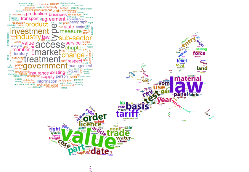
Wordclouds are a commonly used way to display how many times each word is occurring in the text. You can easily do this with the wordcloud or wordcloud2 R package. The following code calculates how many times each noun is occurring and plots these in a wordcloud. The wordcloud2 package gives HTML as output and allows also to set a background image like an image of the Canada flag and the EU.

## Word frequencies
x <- ceta$ceta_nouns[, list(n = .N), by = list(word.lemma)]
x <- x[order(x$n, decreasing = TRUE), ]
x <- as.data.frame(x)

## Visualise them with wordclouds
library(wordcloud)
wordcloud(words = x$word.lemma, freq = x$n, max.words = 150, random.order = FALSE, colors = brewer.pal(8, "Dark2"))

library(wordcloud2)
wordcloud2(data = head(x, 700), figPath = "maple_europa_black.png")

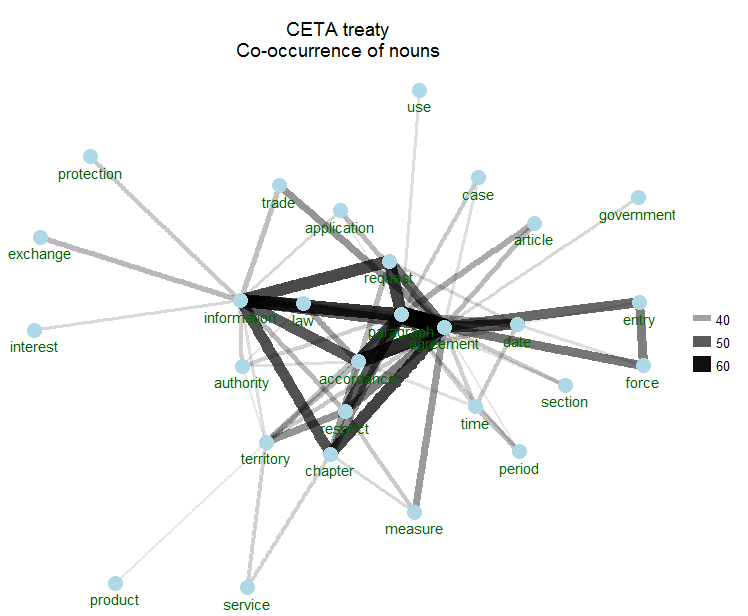
2. But text mining is also about co-occurrence statistics

Co-occurrence statistics indicate how many times 2 words are occuring in the same CETA article. That is great as it gives more indication of how word are used in its context. For this, you can rely on the ggraph & ggforce R packages. The following shows the top 70 word pairs which co-occur and visualises them.

library(ggraph)
library(ggforce)
library(igraph)
library(tidytext)
word_cooccurences <- pair_count(data=ceta$ceta_nouns, group="article.id", value="word.lemma", sort = TRUE)
set.seed(123456789)
head(word_cooccurences, 70) %>%
  graph_from_data_frame() %>%
  ggraph(layout = "fr") +
  geom_edge_link(aes(edge_alpha = n, edge_width = n)) +
  geom_node_point(color = "lightblue", size = 5) +
  geom_node_text(aes(label = name), vjust = 1.8, col = "darkgreen") +
  ggtitle(sprintf("\n%s", "CETA treaty\nCo-occurrence of nouns")) +
  theme_void()

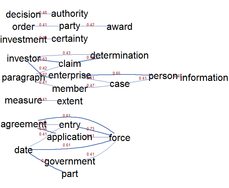
3. And text mining is also about correlations between words

Text mining is also about visualising which words are used next to other words. One can use correlations for that which can be visualised. The following graph shows the top 25 correlations of the words emmitted by topic 3 (the Mr Magnette topic which generated some media fuzz). It shows the words emitted by topic 3, these are words like: claim, dispute, investment certainty, enterprise, decision and authorit ). This correlation visualisation clearly shows the correlations between the words which got into the news recently namely investor claims of enterprises, investment certainties, who is deciding on that and when does this new type of procedure get into place.

library(topicmodels.utils)
idx <- predict(ceta_topics, dtm, type = "topics")
idx <- idx$topic == 3
termcor <- termcorrplot(dtm[idx, ], 
                        words = names(ceta_topic_terms$topic3), highlight = head(names(ceta_topic_terms$topic3), 3),
                        autocorMax = 25, lwdmultiplier = 3, drawlabel = TRUE, cex.label = 0.8) 

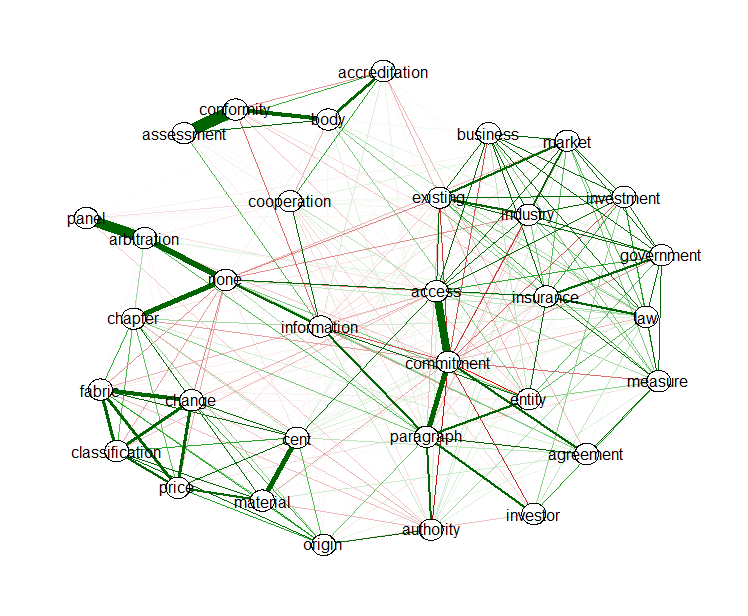
In text mining, you have a lot of terms, you can reduce the many word links to relevant links with the EBICglasso function from the qgraph package. This function allows to reduce the correlation matrix between the words to a similar matrix where correlations which are not relevant are set as much as possible to zero so that these do not need to be visualised. The following R code does this and visualises the positive (green) and negative (red) correlations which are left in the correlation matrix of words emmited by all topics. There is clearly and accreditation body which assess conformity according to regulations, an arbitration panel, and a lot is linked to each other regarding access to the market and the government which ensures the legality of the agreement.

library(Matrix)
library(qgraph)
terms <- predict(ceta_topics, type = "terms", min_posterior = 0.025)
terms <- unique(unlist(sapply(terms, names)))
out <- dtm[, terms]
out <- cor(as.matrix(out))
out <- nearPD(x=out, corr = TRUE)$mat
out <- as.matrix(out)

m <- EBICglasso(out, n = 1000)
qgraph(m, layout="spring", labels = colnames(out), label.scale=FALSE,
       label.cex=1, node.width=.5)

4. If you think of it, words are basically also a network which can be visualised

R packages semnet and visNetwork are your friends here. Words which occur next to each other or within a certain window can be extracted and visualised. Package semnet uses the igraph package for this, package visNetwork allows to generate HTML output to be published on websites. Example graphs are shown below.

library(semnet)
terms <- unique(unlist(sapply(ceta_topic_terms, names)))
cooc <- coOccurenceNetwork(dtm[, terms])
cooc <- simplify(cooc)
plot(cooc, vertex.size=V(cooc)$freq / 20, edge.arrow.size=0.5)

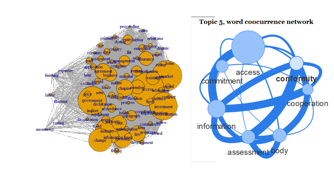
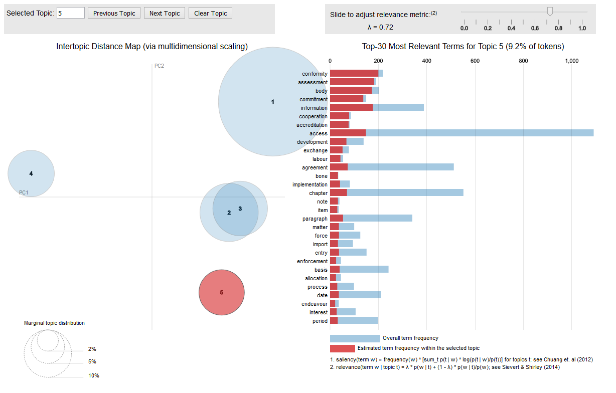
5. And of course you can find topics and visualise these topics

If you are interested in topic models, like the one fitted on the CETA treaty, you should have a look at the excellent LDAvis package which allows you to interactively explore the most salient words that each topic emits and as well visualises the distance between the topics.
The visualisation is interactive and can be put into a web application easily. The following call to the createJSON and serVis R functions from the LDAvis package give you an interactive topic visualisation in no time.

library(LDAvis)
json <- createJSON(phi = posterior(ceta_topics)$terms,
                   theta = posterior(ceta_topics)$topics,
                   doc.length = row_sums(dtm),
                   vocab = colnames(dtm),
                   term.frequency = col_sums(dtm))
serVis(json)

Hope this triggers you a bit to do text mining with R.

If you are interested in all of this, you might be interested also in attending our course on Text mining with R.

Our next course on Text Mining with R is scheduled on 2016 November 14/15 in Brussels (Belgium): more info + register at http://di-academy.com/event/text-mining-with-r/
Our next course on Text Mining with R is scheduled on 2017 March 23/24 in Leuven (Belgium): more info + register at https://lstat.kuleuven.be/training/coursedescriptions/text-mining-with-r

BelgiumMaps.StatBel: R package with Administrative boundaries of Belgium

We recently opened up the BelgiumMaps.StatBel package and made it available at https://github.com/bnosac/BelgiumMaps.StatBel. This R package contains maps with administrative boundaries (national, regions, provinces, districts, municipalities, statistical sectors, agglomerations (200m)) of Belgium extracted from Open Data at Statistics Belgium. 

The package is a data-only package where maps of administrative zones in Belgium are available in the WGS84 coordinate reference system. The data is available in several objects:

• BE_ADMIN_SECTORS: a SpatialPolygonsDataFrame with polygons and data at the level of the statistical sector
• BE_ADMIN_MUNTY: a SpatialPolygonsDataFrame with polygons and data at the level of the municipality
• BE_ADMIN_DISTRICT: a SpatialPolygonsDataFrame with polygons and data at the level of the district
• BE_ADMIN_PROVINCE: a SpatialPolygonsDataFrame with polygons and data at the level of the province
• BE_ADMIN_REGION: a SpatialPolygonsDataFrame with polygons and data at the level of the region
• BE_ADMIN_BELGIUM: a SpatialPolygonsDataFrame with polygons and data at the level of the whole of Belgium
• BE_ADMIN_HIERARCHY: a data.frame with administrative hierarchy of Belgium
• BE_ADMIN_AGGLOMERATIONS: a SpatialPolygonsDataFrame with polygons and data at the level of an agglomeration (200m)

The R package is available at our rcube at www.datatailor.be under the CC-BY 2 license and can be installed as follows:

install.packages("sp")
install.packages("BelgiumMaps.StatBel", repos = "http://www.datatailor.be/rcube", type = "source")

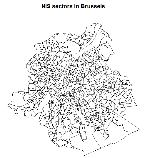
The core data of the package contains administrative boundaries at the level of the statistical sector which can easily be plotted using the sp or the leaflet package.

library(BelgiumMaps.StatBel)
data(BE_ADMIN_SECTORS)
bxl <- subset(BE_ADMIN_SECTORS, TX_RGN_DESCR_NL %in% "Brussels Hoofdstedelijk Gewest")
plot(bxl, main = "NIS sectors in Brussels")

All municipalities, districts, provinces, regions and country level boundaries are also directly available in the package.

data(BE_ADMIN_SECTORS)
data(BE_ADMIN_MUNTY)
data(BE_ADMIN_DISTRICT) 
data(BE_ADMIN_PROVINCE) 
data(BE_ADMIN_REGION) 
data(BE_ADMIN_BELGIUM) 
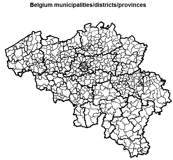
plot(BE_ADMIN_MUNTY, main = "Belgium municipalities/districts/provinces")
plot(BE_ADMIN_DISTRICT, lwd = 2, add = TRUE)
plot(BE_ADMIN_PROVINCE, lwd = 3, add = TRUE)

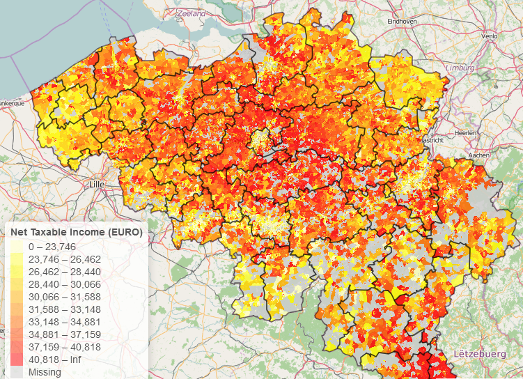
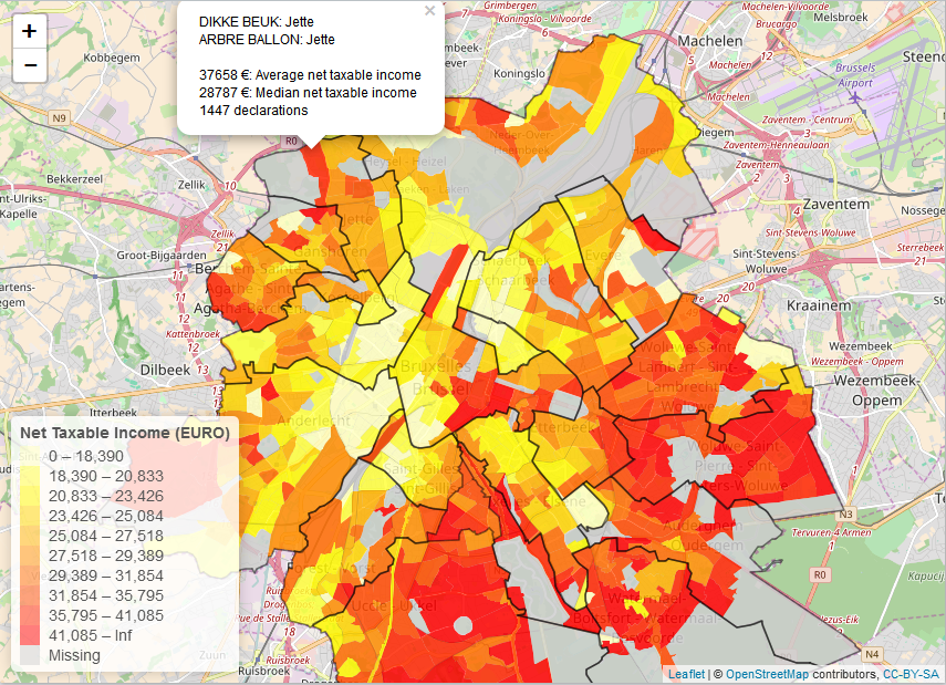
The package also integrates well with other public data from Statistics Belgium as it contains spatial identifiers (nis codes, nuts codes) which you can use to link to other datasets. The following R code example creates an interactive map displaying net taxable income by statistical code for Brussels.

If you are looking for mapping data about Belgium, you might also be interested in the BelgiumStatistics package (which can be found at https://github.com/weRbelgium/BelgiumStatistics) containing more general statistics about Belgium or the BelgiumMaps.OpenStreetMap package (https://github.com/weRbelgium/BelgiumMaps.OpenStreetMap) which contains geospatial data of Belgium regarding landuse, natural, places, points, railways, roads and waterways, extracted from OpenStreetMap.

library(BelgiumMaps.StatBel)
library(leaflet)

## Get taxes / statistical sector
tempfile <- tempfile()
download.file("http://statbel.fgov.be/nl/binaries/TF_PSNL_INC_TAX_SECTOR_tcm325-278417.zip", tempfile)
unzip(tempfile, list = TRUE)
taxes <- read.table(unz(tempfile, filename = "TF_PSNL_INC_TAX_SECTOR.txt"), sep="|", header = TRUE, encoding = "UTF-8", stringsAsFactors = FALSE, quote = "", na.strings = c("", "C"))
colnames(taxes)[1] <- "CD_YEAR"

## Get taxes in last year
taxes <- subset(taxes, CD_YEAR == max(taxes$CD_YEAR))
taxes <- taxes[, c("CD_YEAR", "CD_REFNIS_SECTOR", 
"MS_NBR_NON_ZERO_INC", "MS_TOT_NET_TAXABLE_INC", "MS_AVG_TOT_NET_TAXABLE_INC", 
"MS_MEDIAN_NET_TAXABLE_INC", "MS_INT_QUART_DIFF", "MS_INT_QUART_COEFF", 
"MS_INT_QUART_ASSYM")]

## Join taxes with the map
data(BE_ADMIN_SECTORS, package = "BelgiumMaps.StatBel")
data(BE_ADMIN_DISTRICT, package = "BelgiumMaps.StatBel")
data(BE_ADMIN_MUNTY, package = "BelgiumMaps.StatBel")
str(BE_ADMIN_SECTORS@data)
mymap <- merge(BE_ADMIN_SECTORS, taxes, by = "CD_REFNIS_SECTOR", all.x=TRUE, all.y=FALSE)
mymap <- subset(mymap, TX_RGN_DESCR_NL %in% "Brussels Hoofdstedelijk Gewest")

## Visualise the data
pal <- colorBin(palette = rev(heat.colors(11)), domain = mymap$MS_AVG_TOT_NET_TAXABLE_INC,
bins = c(0, round(quantile(mymap$MS_AVG_TOT_NET_TAXABLE_INC, na.rm=TRUE, probs = seq(0.1, 0.9, by = 0.1)), 0), +Inf),
na.color = "#cecece")

m <- leaflet(mymap) %>%
  addTiles() %>%
  addLegend(title = "Net Taxable Income (EURO)", 
    pal = pal, values = ~MS_AVG_TOT_NET_TAXABLE_INC, 
    position = "bottomleft", na.label = "Missing") %>%
  addPolygons(color = ~pal(MS_AVG_TOT_NET_TAXABLE_INC), 
   stroke = FALSE, smoothFactor = 0.2, fillOpacity = 0.85,
   popup = sprintf("%s: %s<br>%s: %s<br><br>%s €: Average net taxable income<br>%s €: Median net taxable income<br>%s declarations", 
     mymap$TX_SECTOR_DESCR_NL, mymap$TX_MUNTY_DESCR_NL, 
     mymap$TX_SECTOR_DESCR_FR, mymap$TX_MUNTY_DESCR_FR,  
     mymap$MS_AVG_TOT_NET_TAXABLE_INC, mymap$MS_MEDIAN_NET_TAXABLE_INC, 
     mymap$MS_NBR_NON_ZERO_INC))
#m <- addPolylines(m, data = BE_ADMIN_DISTRICT, weight = 1.5, color = "black")
m <- addPolylines(m, data = subset(BE_ADMIN_MUNTY, 
  TX_RGN_DESCR_NL %in% "Brussels Hoofdstedelijk Gewest"), weight = 1.5, color = "black")
m