Last week, OpenAI released version 2 of an updated neural net called Whisper that approaches human level robustness and accuracy on speech recognition. You can now directly call from R a C/C++ inference engine which allow you to transcribe .wav audio files.
library(audio.whisper)
model <- whisper("tiny")
path  <- system.file(package = "audio.whisper", "samples", "jfk.wav")
trans <- predict(model, newdata = path, language = "en", n_threads = 2)
trans
$n_segments
[1] 1

$data
 segment         from           to                                                                                                       text
       1 00:00:00.000 00:00:11.000  And so my fellow Americans ask not what your country can do for you ask what you can do for your country.

$tokens
 segment      token token_prob
       1        And  0.7476438
       1         so  0.9042299
       1         my  0.6872202
       1     fellow  0.9984470
       1  Americans  0.9589157
       1        ask  0.2573057
       1        not  0.7678108
       1       what  0.6542882
       1       your  0.9386917
       1   counstry  0.9854987
       1        can  0.9813995
       1         do  0.9937403
       1        for  0.9791515
       1        you  0.9925495
       1        ask  0.3058807
       1       what  0.8303462
       1        you  0.9735528
       1        can  0.9711444
       1         do  0.9616748
       1        for  0.9778513
       1       your  0.9604713
       1    country  0.9923630
       1          .  0.4983074
Another example based on a Micro Machines commercial from the 1980's.
This week, I uploaded a newer version of the R package recogito to CRAN.
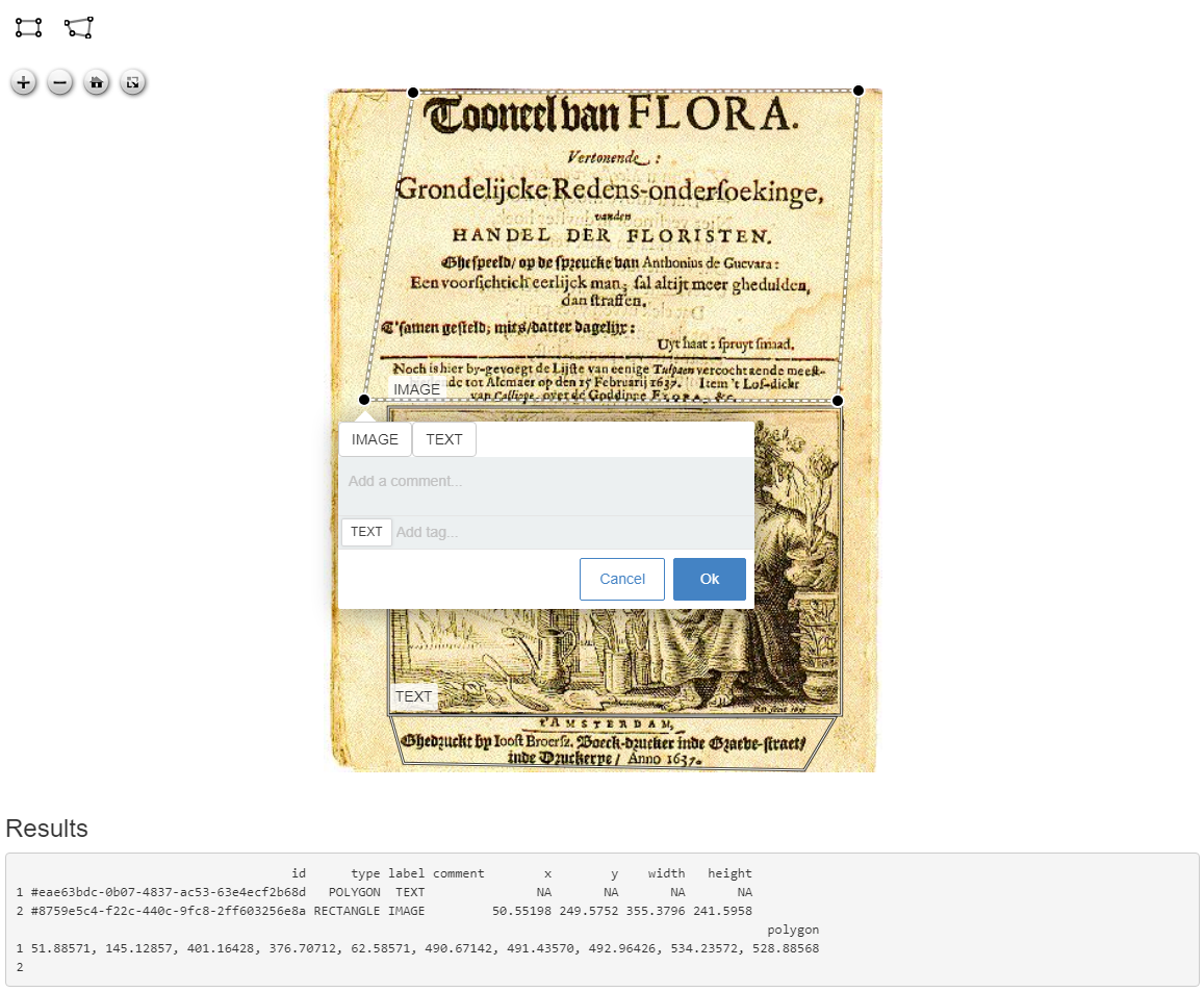
The recogito R package provides tools to manipulate and annotate images and text in shiny. It is a htmlwidgets R wrapper around the excellent recogito-js and annotorious javascript libraries as well as it's integration with openseadragon. You can use the package to set up shiny apps which
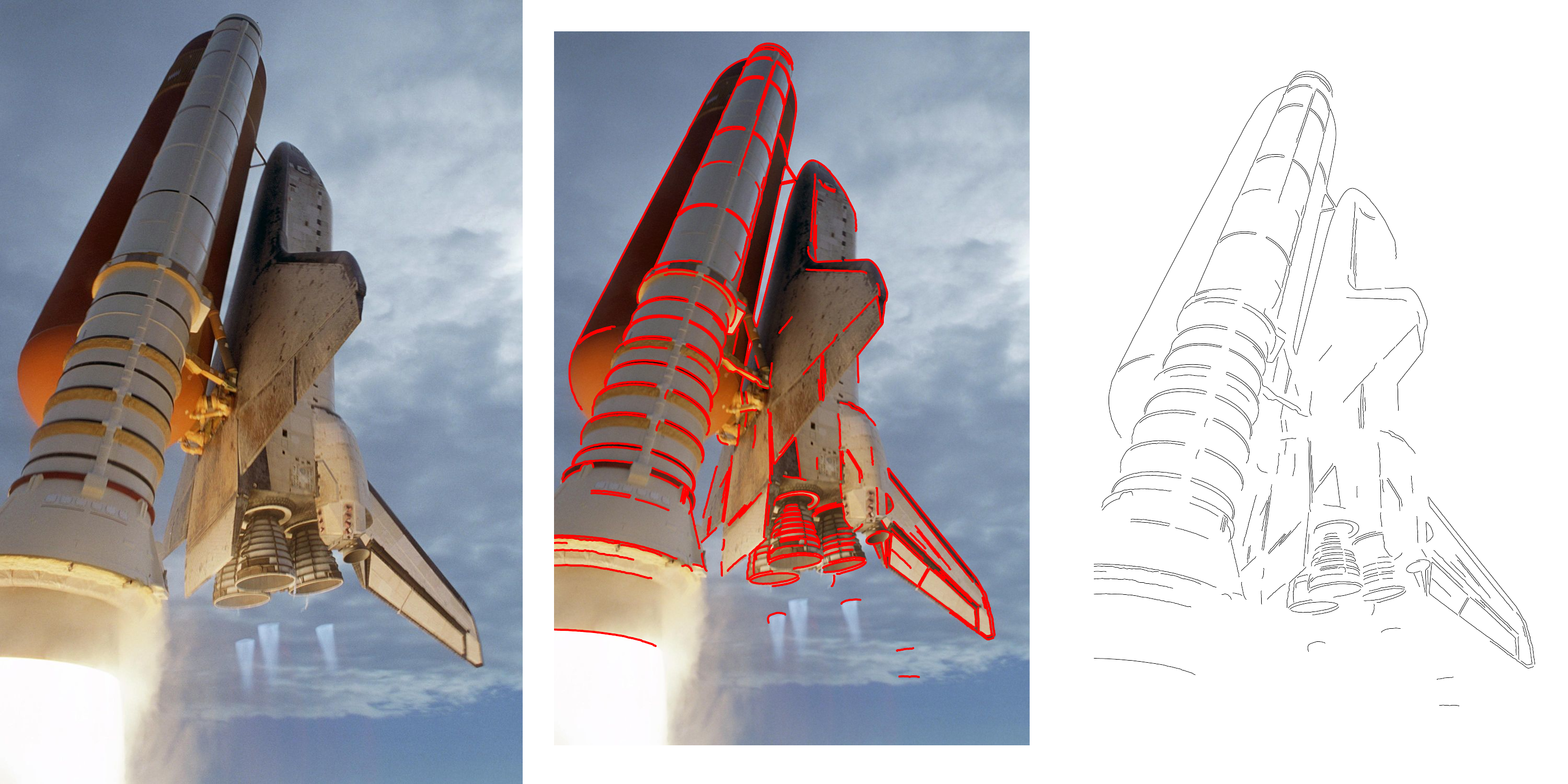
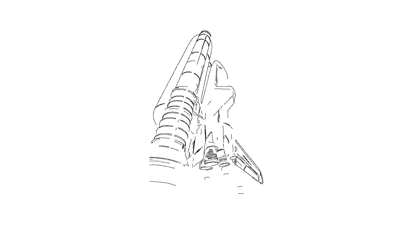
annotate areas of interest (rectangles / polygons) in images with specific labels
annotate text using tags and relations between these tags (for entity labelling / entity linking).
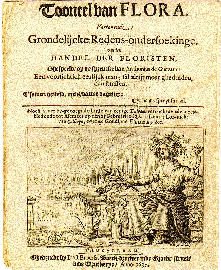
The video below shows the image manipulation functionality in action in a shiny app which allows to align image areas with chunks of transcribed handwritten texts.
Although the package was orginally designed to extract information from handwritten text documents from the 18th-19th century, you can probably use it in other domains as well. To get you started install the package from CRAN and read the README.
install.packages("recogito")
The following code shows an example app which shows an url and allows you to annotate areas of interest. Enjoy.
NEW, since 2020, you can now access courses Text Mining with R and Advanced R programming online through our online school, let us know here if you want to obtain access.
An update of the udpipe R package (https://bnosac.github.io/udpipe/en) landed safely on CRAN last week. Originally the udpipe R package was put on CRAN in 2017 wrapping the UDPipe (v1.2 C++) tokeniser/lemmatiser/parts of speech tagger and dependency parser. It now has many more functionalities next to just providing this parser.
The current release (0.8.4-1 on CRAN: https://cran.r-project.org/package=udpipe) makes sure default models which are used are the ones trained on version 2.5 of universal dependencies. Other features of the release are detailed in the NEWS item. This is what dependency parsing looks like on some sample text.
library(udpipe)
x <- udpipe("The package provides a dependency parsers built on data from universaldependencies.org", "english")
View(x)
library(ggraph)
library(ggplot2)
library(igraph)
library(textplot)
plt <- textplot_dependencyparser(x, size = 4, title = "udpipe R package - dependency parsing")
plt
During the years, the toolkit has now also incorporated many functionalities for commonly used data manipulations on texts which are enriched with the output of the parser. Namely functionalities and algorithms for collocations, token co-occurrence, document term matrix handling, term frequency inverse document frequency calculations, information retrieval metrics, handling of multi-word expressions, keyword detection (Rapid Automatic Keyword Extraction, noun phrase extraction, syntactical patterns) sentiment scoring and semantic similarity analysis.
Many add-on R packages
The udpipe package is loosely coupled with other NLP R packages which BNOSAC released in the last 4 years on CRAN. Loosely coupled means that none of the packages have hard dependencies of one another making it easy to install and maintain and allowing you to use only the packages and tools that you want.
Hereby a small list of loosely coupled packages by BNOSAC which contain functions and documentation where the udpipe package is used as a preprocessing step.
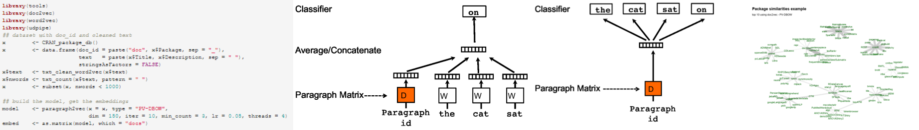
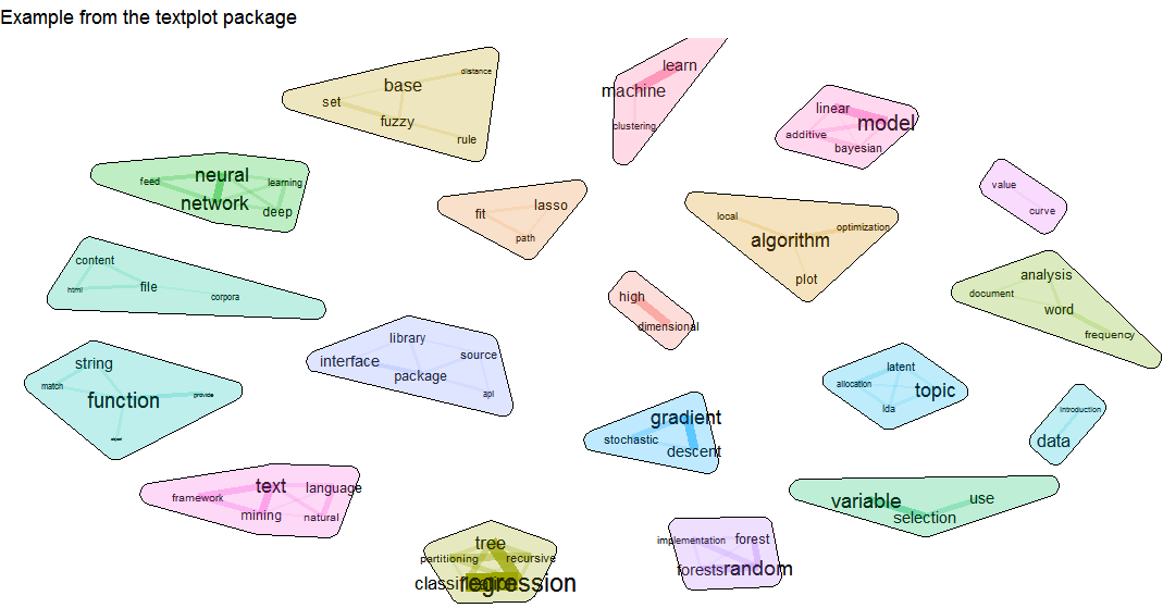
- BTM: Biterm Topic Modelling - crfsuite: Build named entity recognition models using conditional random fields - nametagger: Build named entity recognition models using markov models - torch.ner: Named Entity Recognition using torch - word2vec: Training and applying the word2vec algorithm - ruimtehol: Text embedding techniques using Starspace - textrank: Text summarisation and keyword detection using textrank - brown: Brown word clustering on texts - sentencepiece: Byte Pair Encoding and Unigram tokenisation using sentencepiece - tokenizers.bpe: Byte Pair Encoding tokenisation using YouTokenToMe - text.alignment: Find text similarities using Smith-Waterman - textplot: Visualise complex relations in texts
Model building example
To showcase the loose integration, let's use the udpipe package alongside the word2vec package to build a udpipe model by ourselves on the German GSD treebank which is described at https://universaldependencies.org/treebanks/de_gsd/index.html and contains a set of CC BY-SA licensed annotated texts from news articles, wiki entries and reviews. More information at https://universaldependencies.org.
Note that model training takes a while (8hours up to 3days) depending on the size of the treebank and your hyperparameter settings. This example was run on a Windows i5 CPU laptop with 1.7Ghz, so no GPU needed, which makes this model building process still accessible for anyone with a simple PC.
You can see the logs of this run here. Now your model is ready, you can use it on your own terms and you can start using it to annotate your text.
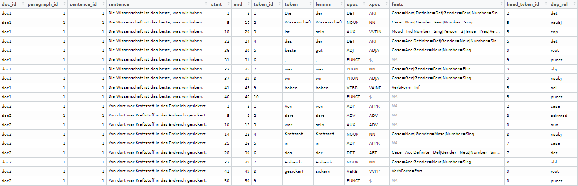
model <- udpipe_load_model("de_gsd-ud-2.6-20200924.udpipe")
texts <- data.frame(doc_id = c("doc1", "doc2"), text = c("Die Wissenschaft ist das beste, was wir haben.", "Von dort war Kraftstoff in das Erdreich gesickert."), stringsAsFactors = FALSE)
anno  <- udpipe(texts, model, trace = 10)
View(anno)
Enjoy!
Thanks to Slav Petrov, Wolfgang Seeker, Ryan McDonald, Joakim Nivre, Daniel Zeman, Adriane Boyd for creating and distributing the UD_German-GSD treebank and to the UDPipe authors in particular Milan Straka.
 You can view the presentation below.
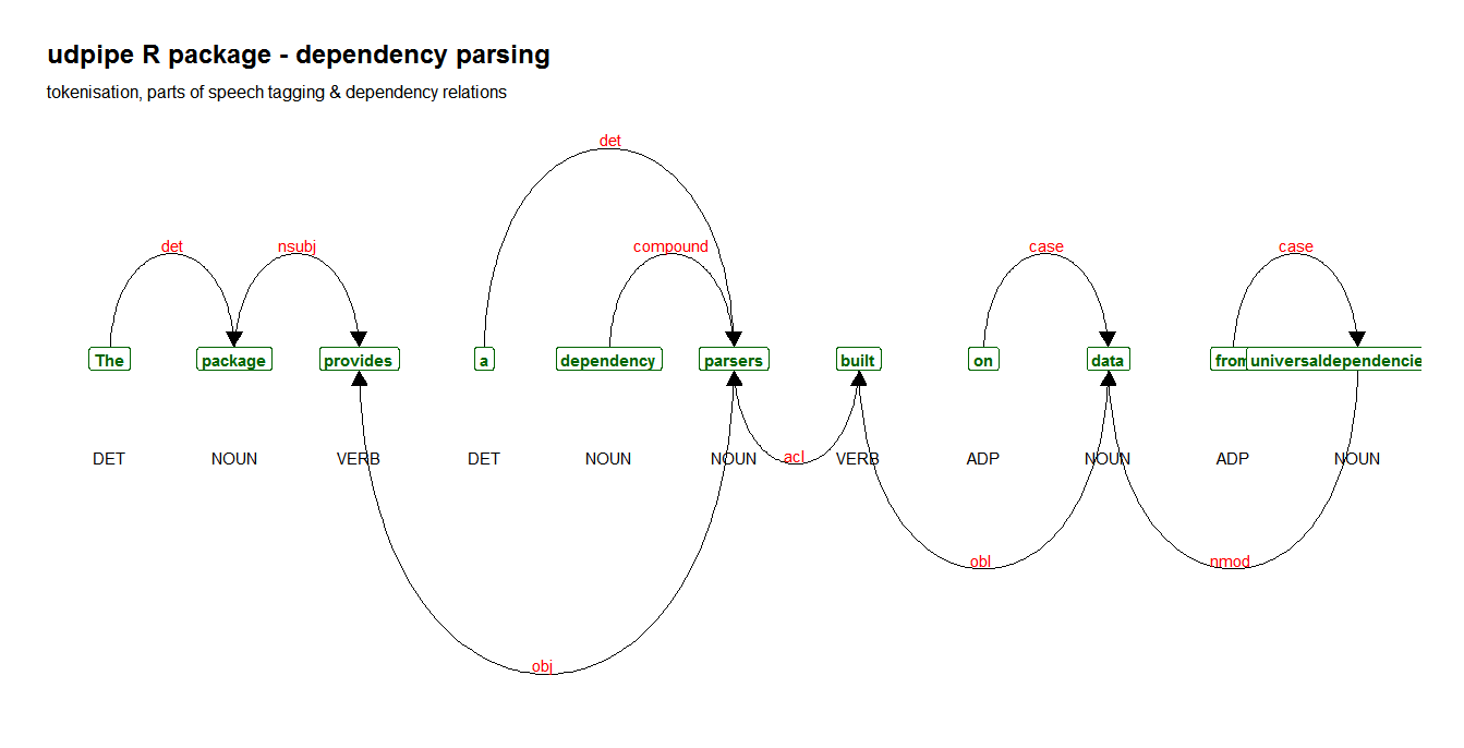
